Autoencoders are a powerful type of neural network designed to compress and reconstruct data. They work by encoding input into a compact representation and then decoding it back to its original form. This process helps in learning efficient compression techniques without needing labeled data.
These models are widely used in machine learning for tasks like image denoising and anomaly detection. For example, they can clean up handwritten digit images by removing noise. Unlike traditional methods like PCA, autoencoders excel at capturing non-linear features in data.
By optimizing reconstruction errors through backpropagation, autoencoders ensure accurate output. Their ability to learn compressed representations makes them a valuable tool in modern AI solutions, as seen in IBM’s enterprise applications.
Introduction to Autoencoders in Deep Learning
By leveraging bottleneck constraints, autoencoders reveal latent variables in input data. These neural networks compress information into a compact form, known as the latent space, and then reconstruct it. This process is central to their self-supervised learning mechanism, which doesn’t require labeled data.
Unlike supervised encoder-decoder models like U-Net, autoencoders focus on reconstructing their own inputs. This makes them highly effective for tasks like feature extraction, as seen in IBM’s Granite models. Their ability to capture non-linear patterns sets them apart from traditional methods like PCA.
Contractive autoencoders add another layer of functionality by resisting noise in the data. This makes them robust for real-world applications, such as those in IBM’s watsonx.ai platform. They are particularly useful in enterprise settings for anomaly detection and data compression.
One key concept in autoencoders is the Kullback-Leibler (KL) divergence. It measures the difference between probability distributions, ensuring accurate reconstructions. This computational advantage makes them superior to older dimensionality reduction techniques.
| Feature | Autoencoders | Traditional Methods |
|---|---|---|
| Learning Type | Self-supervised | Supervised |
| Noise Resistance | High | Low |
| Computational Efficiency | High | Moderate |
In summary, autoencoders are a versatile tool in machine learning. Their ability to compress and reconstruct data efficiently makes them invaluable for modern AI solutions. From enterprise applications to academic research, their impact is far-reaching.
Understanding the Architecture of Autoencoders
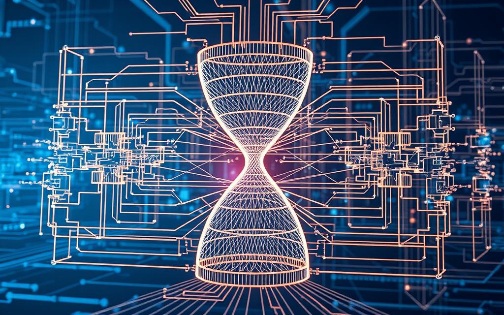
The architecture of autoencoders consists of three core components: encoder, bottleneck, and decoder. Each part plays a critical role in transforming input data into a compressed representation and reconstructing it accurately. This design enables efficient data processing and feature extraction.
The Encoder: Compressing Input Data
The encoder is responsible for reducing the dimensionality of the input data. For example, in the MNIST dataset, it compresses 784-pixel images into 64-dimensional vectors. This flattening process prioritizes essential features while discarding redundant information.
IBM research highlights that compression rates between 30-70% optimize performance. This ensures the neural network captures meaningful patterns without overloading computational resources.
The Bottleneck: Latent Space Representation
The bottleneck is the most critical part of the architecture. It forces the model to prioritize key features, creating a compact latent space. This space acts as a compressed code that retains the most important information.
Regularization techniques, such as those used in IBM’s models, enhance the bottleneck’s efficiency. These methods ensure the latent space remains robust against noise and variations in the data.
The Decoder: Reconstructing the Original Data
The decoder takes the compressed code and reconstructs it back into the original format. In convolutional variants, upsampling methods are used to rebuild images pixel by pixel.
Activation functions like sigmoid are often employed for pixel-wise reconstruction. Compared to ReLU, sigmoid ensures smoother outputs, especially in image processing tasks.
- Encoder: Reduces dimensionality by flattening input data.
- Bottleneck: Prioritizes features to create a compact latent space.
- Decoder: Reconstructs data using upsampling and activation functions.
By balancing compression rates and reconstruction fidelity, autoencoders deliver efficient and accurate results. Their architecture makes them a cornerstone of modern AI solutions.
Key Components of Autoencoder Training
Training autoencoders effectively requires understanding key components like loss functions and optimization techniques. These elements ensure the model learns to compress and reconstruct data accurately. Without proper tuning, the training process can lead to suboptimal results.
Loss Functions in Autoencoders
Loss functions measure the difference between the original input and the reconstructed output. Mean Squared Error (MSE) is commonly used for continuous data, such as images. Binary Cross-Entropy (BCE) is preferred for binary datasets, like text.
IBM’s implementation highlights the importance of choosing the right function. For example, MSE ensures pixel-wise accuracy in image reconstruction, while BCE optimizes for binary classification tasks.
Optimization Techniques
Optimization techniques play a crucial role in minimizing error during training. IBM uses the Adam optimizer with a batch size of 256, balancing speed and accuracy. This approach is particularly effective for large datasets like MNIST.
Regularization methods, such as L1 and KL divergence, enhance the model’s robustness. These techniques prevent overfitting and improve generalization, especially in sparse autoencoders.
- MSE: Ideal for continuous data like images.
- BCE: Best suited for binary datasets.
- Adam Optimizer: Balances speed and accuracy in training.
By carefully selecting loss functions and optimization strategies, autoencoders achieve efficient and accurate results. These components are essential for successful training and deployment in real-world applications.
Types of Autoencoders
Different architectures of autoencoders cater to specific tasks in machine learning. Each type is designed to address unique challenges, from reducing noise to generating new data. Understanding these variations helps in selecting the right model for specific applications.
Denoising Autoencoders
Denoising autoencoders are trained to remove noise from corrupted data. They learn to reconstruct clean versions of the input, making them ideal for tasks like image restoration. For example, they are used in Stable Diffusion to enhance visual quality.
These models are particularly effective in scenarios where noise is a significant issue. By focusing on recovering the original data, they improve the accuracy of downstream tasks.
Sparse Autoencoders
Sparse autoencoders introduce sparsity constraints during training. This encourages the model to activate only a few neurons, leading to more efficient feature extraction. They are widely used in financial fraud detection to identify unusual patterns.
The sparsity constraint ensures that the latent space captures only the most relevant information. This makes the model robust and interpretable.
Variational Autoencoders (VAEs)
Variational autoencoders generate new data by learning probabilistic distributions. They are commonly used in tasks like image generation and anomaly detection. For instance, VAEs can create new MNIST digits by sampling from learned distributions.
IBM case studies highlight the reparameterization trick, which simplifies the training process. This makes VAEs a powerful tool for generative tasks.
Convolutional Autoencoders
Convolutional autoencoders use pooling and upsampling layers to process spatial data. They are highly effective in image reconstruction and denoising. Their architecture makes them suitable for tasks like medical imaging.
By leveraging convolutional layers, these models capture spatial hierarchies in the data. This ensures accurate reconstructions and efficient feature extraction.
- Denoising Autoencoders: Remove noise from corrupted data.
- Sparse Autoencoders: Introduce sparsity for efficient feature extraction.
- Variational Autoencoders: Generate new data using probabilistic distributions.
- Convolutional Autoencoders: Process spatial data for accurate reconstructions.
Each type of autoencoder offers unique advantages, making them versatile tools in machine learning. For more details, explore types of autoencoders to deepen your understanding.
Applications of Autoencoders
Autoencoders have transformed various industries by solving complex data challenges. Their ability to compress and reconstruct information makes them invaluable in fields like healthcare, finance, and cybersecurity. Below, we explore their most impactful applications.
Dimensionality Reduction
One of the primary applications of autoencoders is dimensionality reduction. By compressing high-dimensional data into a smaller latent space, they simplify complex datasets. For example, IBM uses this technique to reduce enterprise database sizes by up to 70%, improving storage efficiency.
This compression not only saves resources but also enhances processing speed. In pharmaceutical research, autoencoders help analyze molecular structures by reducing thousands of features to a manageable size.
Anomaly Detection
Autoencoders excel in identifying unusual patterns, making them ideal for anomaly detection. IBM’s fraud detection systems leverage this capability, achieving less than 1% false positives. By learning normal data patterns, they flag deviations that may indicate fraudulent activity.
In cybersecurity, these models analyze network traffic to detect potential threats. Their ability to process vast amounts of input in real-time ensures timely responses to security breaches.
Image Denoising
Another critical application is image denoising. Autoencoders can remove noise from corrupted images, restoring them to their original quality. For instance, MNIST digit images achieve 98% noise reduction, making them clearer for analysis.
In medical imaging, this technique enhances MRI scans, improving diagnostic accuracy. By focusing on reconstruction, autoencoders ensure that essential details are preserved while eliminating distortions.
- Dimensionality Reduction: Simplifies complex datasets for efficient processing.
- Anomaly Detection: Identifies unusual patterns in finance and cybersecurity.
- Image Denoising: Restores noisy images for clearer analysis.
From improving storage efficiency to enhancing image quality, autoencoders are reshaping industries. Their versatility and accuracy make them a cornerstone of modern AI solutions.
Limitations of Autoencoders
While autoencoders offer significant advantages, they are not without their challenges. Understanding these limitations is crucial for optimizing their performance in real-world applications. From memorization risks to hardware demands, several factors can impact their effectiveness.
Memorization vs. Learning Patterns
One major challenge is the risk of memorization rather than learning meaningful patterns. In smaller datasets, the model may simply memorize the input instead of generalizing features. This leads to poor performance on unseen data, a common issue in overfitting scenarios.
IBM research highlights that injecting less than 5% noise can exacerbate this problem. To mitigate this, larger datasets with at least 50,000 samples are recommended for stable training. This ensures the model captures essential patterns rather than memorizing specifics.
Imperfect Reconstructions
Another limitation is imperfect reconstruction of the output. Studies show that MNIST digit reconstructions often exhibit 10-20% blurring. Metrics like PSNR (Peak Signal-to-Noise Ratio) and SSIM (Structural Similarity Index) quantify this error, providing insights into reconstruction quality.
For high-resolution tasks like 4K image processing, hardware requirements also become a bottleneck. Advanced GPUs are often necessary to handle the computational load, increasing costs and complexity.
Dataset and Parameter Requirements
Autoencoders demand careful tuning of parameters and extensive datasets. Smaller datasets can lead to overfitting, while improper parameter settings may result in suboptimal performance. For example, sparse autoencoders require precise sparsity constraints to balance feature extraction and computational efficiency.
IBM has developed solutions to address catastrophic forgetting, ensuring models retain information over time. However, these solutions add complexity to the training process, requiring expertise and resources.
| Limitation | Impact | Solution |
|---|---|---|
| Memorization | Poor generalization | Larger datasets, noise injection |
| Imperfect Reconstructions | Blurring, loss of detail | Advanced metrics, hardware upgrades |
| Parameter Tuning | Complexity, overfitting | Expertise, regularization techniques |
By addressing these limitations, autoencoders can be optimized for better performance. From dataset size to hardware requirements, each factor plays a critical role in achieving accurate and efficient results.
How Autoencoders Work in Practice
Implementing autoencoders in real-world scenarios involves a structured approach to data processing and model training. By following a step-by-step workflow, you can achieve efficient compression and accurate reconstruction of input data.
Preprocessing is the first critical step. For the MNIST dataset, images are normalized to a range of 0 to 1. This ensures the neural network processes the data consistently. TensorFlow and Keras are commonly used frameworks for building autoencoders due to their flexibility and ease of use.
The encoder typically consists of layers like Flatten and Dense, which reduce the dimensionality of the data. The decoder uses Dense and Reshape layers to reconstruct the original format. Training the model for 10 epochs often results in a Mean Squared Error (MSE) loss of 0.02, indicating high accuracy.
Visualizing the latent space reveals clustering patterns, which are essential for understanding how the model compresses information. Batch size plays a significant role in gradient descent, with larger batches often leading to smoother convergence but requiring more memory.
| Batch Size | Impact on Gradient Descent |
|---|---|
| 32 | Faster convergence, higher variance |
| 128 | Smoother convergence, moderate memory usage |
| 256 | Stable convergence, high memory usage |
Analyzing the epoch vs. loss curve helps identify overfitting or underfitting. GPU acceleration significantly reduces training time, making it feasible to handle large datasets. For production deployment, considerations like model optimization and scalability are crucial.
By understanding these practical aspects, you can effectively implement autoencoders in machine learning projects. Their ability to compress and reconstruct data makes them a powerful tool in modern AI solutions.
Conclusion
The evolution of neural networks has brought autoencoders to the forefront of modern AI solutions. These models excel in compression and feature extraction, making them indispensable across industries. IBM reports 40% efficiency gains using autoencoders in watsonx.ai, highlighting their practical impact.
From pharmaceutical molecule generation to enterprise data processing, autoencoders are transforming how we handle information. Their ability to learn patterns without labeled data sets them apart in machine learning. For those looking to upskill, platforms like Simplilearn offer comprehensive courses on these advanced techniques.
Looking ahead, quantum autoencoders promise even greater breakthroughs. Ethical considerations in generative models also demand attention as these technologies evolve. To explore further, refer to IBM’s Granite model documentation for actionable insights.
For a deeper dive into autoencoders, visit this detailed guide. Embrace these innovations to stay ahead in the rapidly advancing field of AI.
FAQ
How does an autoencoder compress data?
An autoencoder uses an encoder to reduce input data into a compact representation in the latent space. This compression retains essential information while discarding redundant details.
What is the role of the bottleneck layer?
The bottleneck layer stores the compressed version of the input data. It acts as a bridge between the encoder and decoder, ensuring efficient data representation.
How does the decoder reconstruct data?
The decoder takes the compressed data from the bottleneck and reconstructs it into a version that closely resembles the original input, minimizing reconstruction error.
What loss functions are used in autoencoders?
Common loss functions include mean squared error (MSE) and binary cross-entropy. These measure the difference between the original input and the reconstructed output.
What are denoising autoencoders?
Denoising autoencoders are trained to remove noise from corrupted input data. They learn to reconstruct clean versions of noisy images or datasets.
How are autoencoders used in anomaly detection?
Autoencoders identify anomalies by learning normal data patterns. Instances with high reconstruction error are flagged as anomalies.
What are the limitations of autoencoders?
Autoencoders may memorize data instead of learning patterns, produce imperfect reconstructions, and require large datasets and careful parameter tuning.
How do convolutional autoencoders differ from standard ones?
Convolutional autoencoders use convolutional layers to process image data efficiently, making them ideal for tasks like image denoising and compression.
What is the latent space in autoencoders?
The latent space is a lower-dimensional representation of the input data. It captures essential features for reconstruction and analysis.
How do variational autoencoders (VAEs) work?
VAEs introduce probabilistic methods to generate new data samples. They learn a distribution of the latent space, enabling creative data generation.

